2 SmartScale API
Developed by Jameson Brennan, Ira Parsons, and Hector Menendez Department of Animal Science, South Dakota State University
The objectives of this hands on tutorial are to introduce workshop participants to methods for streamlining SmartScale data processing tasks in R.
2.1 API
2.1.1 Libraries
Our first step to processing the data is to import the libraries we will use to run our analysis. Each library contains a set of functions which can be used to process data. For example, the function mean() would sum the values in a column and divide by the number of observations in the column. This code will look to see if the necessary packages are installed on your computer and if not install and load them.
##if there is an error and a package or dependency needs to be updated un-comment the
#code below and replace 'rvest' with package
#remove.packages('rvest')
#install.packages('rvest')

#Needed packages
  list.of.packages <- c("rvest",'tidyverse','data.table','lubridate',
                        'knitr','markdown','fasttime','MASS')
  new.packages <- list.of.packages[!(list.of.packages %in%
                                       installed.packages()[,"Package"])]
  if(length(new.packages)) install.packages(new.packages)
library(rvest)
library(tidyverse)
library(data.table)
library(lubridate)
library(knitr)
library(rmarkdown)
library(fasttime)
library(MASS)
2.1.2 Login Variables
The first thing you need to do is to enter your variables for the code to run. In the quotations below you will need to change the username, password, FID (or SmartScale ID), and the start and end times for the data you want to download.
Two things to note are 1) you can enter multiple greenfeeds assocated with an account and 2) the start time and end time must be in the same format. The chunk below sets the end time to the computer time for the most recent downloads.
#change to login user name
USERNAME <- 'demo_user'

#Change to login password
PASSWORD <- 'greenfeed'

#Change SmartScale id or id's. The second line can be uncommented out for multiple
#SmartScales notice there is no space between commas for the multiple id's
SmartScale_ID  <- '1000119'
#SmartScale_ID   <- "1000119,1000121,1000132"

#enter the start date (ST) and end date (ET) for the data you want to download
date.start <- '2023-03-14'
date.end   <- '2023-06-01'

## Data parameters -----
FULL_WEIGHT <- 1 # 1 for full body weight calculated using C-Lock algorithm, 0 for raw
#half-body weights, full weights calculated by taking the front end weight * 1.76
GET_VISITS <- 1 #Put 1 to get individual visits, Put 0 to get daily averages
2.1.3 Data Download
This code chunk will pull the data from the cloud based on the specifications of what was provided above.
# Local system setup ----
## Choose a temp folder to download the CSV to ----
if(Sys.info()["sysname"] == "Darwin"){
  TEMP_DIRECTORY <- "/tmp" #For Mac or Linux
}else{
  TEMP_DIRECTORY <- "."    #For Windows (Maybe put C:\Users\yourusername\Desktop)
}

## Load required libraries ----
suppressWarnings(suppressMessages(try(require(rvest), silent = TRUE)))
suppressWarnings(suppressMessages(try(require(httr), silent = TRUE)))
suppressWarnings(suppressMessages(try(require(RCurl), silent = TRUE)))

## Login URL -----
login_url <- "https://greenfeed.c-lockinc.com/GreenFeed/checklogon.php"

## API URL -----
if (GET_VISITS == GET_VISITS) {
  #Download URL - Individual Visits Weights
  download_url <- paste0("https://greenfeed.c-lockinc.com/GreenFeed/tabledata/sfanimals/getanimalweightdetails.php?dl=1",
                         "&fids=0,", SmartScale_ID,
                         "&st=", date.start,
                         "&et=", date.end,
                         "&full=", FULL_WEIGHT);
} else {
  #Download URL - Daily Average Weights
  download_url <- paste0("https://greenfeed.c-lockinc.com/GreenFeed/tabledata/sfanimals/animalweights.php?dl=1&summary=0",
                         "&fids=0,", SmartScale_ID,
                         "&from=", date.start0,
                         "&to=", date.end,
                         "&full=", FULL_WEIGHT);
}

# Download data ----
## Log into the website using URL requests -----
{
  #Create session then download form data
  session <- session("https://greenfeed.c-lockinc.com/GreenFeed")
  form <- html_form(read_html(login_url))[[1]]

  #Set login credentials
  form <- set_values(form, username = USERNAME)
  form <- set_values(form, password = PASSWORD)
  suppressWarnings(form <- set_values(form, redir = "home.php?logout")) #This will give you a warning - we can hide it with suppressWarnings

  #Save main page url
  suppressMessages(main_page <- submit_form(session, form))

  #Download the data
  download <- jump_to(main_page, download_url)
}

# Decode binary data ----
#Because the downloaded data is binary data, you must write it to a temporary file then read it back as a CSV.
## Write data to a file ----
FILENAME <- paste0(TEMP_DIRECTORY, "/C.txt")
writeBin(download$response$content, FILENAME)

#Read the CSV into a df dataframe
if (GET_VISITS == 1) {
  #SmartScale Headers are: "Link" "StartTime" "StopTime" "FeederID" "Duration" "AnimalName" "RFIDTag" "Weight" "Valid"
  colclasses=c("character", "POSIXct", "POSIXct", "integer", "integer", "character", "character", "integer", "character");
} else {
  #SmartScale Headers are: "Link" "StartTime" "StopTime" "FeederID" "Duration" "AnimalName" "RFIDTag" "Weight" "Valid"
  colclasses=c("character", "character");
}

d.smart = fread(file = FILENAME, header=TRUE, sep=",", quote="\"", colClasses = colclasses) # Read into data.table
d.smart[d.smart == 0] <- NA # Replace 0's with NA
2.2 Data Processing
This is the raw dataset downloaded from the SmartScale API.The code chunk will print the first five rows of data in table format.
We can see that the ‘view’ column is likely not necessary and can be removed. In addition, we will create a new column called ‘Date’ that converts the start time to a Date only value. Lastly we will convert the 14 digit RFID number to only the last 6 digits to simplify identifying unique animals.
#Remove unnecessary columns
d.smart$View=NULL


#convert date time to date value to look at daily visits
d.smart$Date=as.Date(d.smart$StartTime)
d.smart$RFIDTag= stringr:: str_sub(d.smart$RFIDTag,-6,-1) #get last 6 digits of RFID
One of the first steps to processing and cleaning data is to plot it. This code chunk will get the number of daily visits for each scale and plot it by day.
2.3 Data Visualization
This next section is used to generate a series of quick plots to summarize visits and data from the SmartScales to check usage rates. This can be helpful to plot is animals are routinely using the equipment and to see if there are any sudden changes in usage rate that may indicate either a issue with the technology or access.
#get the number of unique animals visiting by day
rfid_day=d.smart %>%                              # Applying group_by & summarise
  group_by(Date,FeederID) %>%
  summarise(count = n_distinct(RFIDTag))


rfid_day=na.omit(rfid_day)

ggplot(rfid_day,aes(x=Date,y=count))+
  geom_bar(stat = 'identity')+
  facet_wrap(~FeederID)+
  ggtitle('Number of Unique animals per day')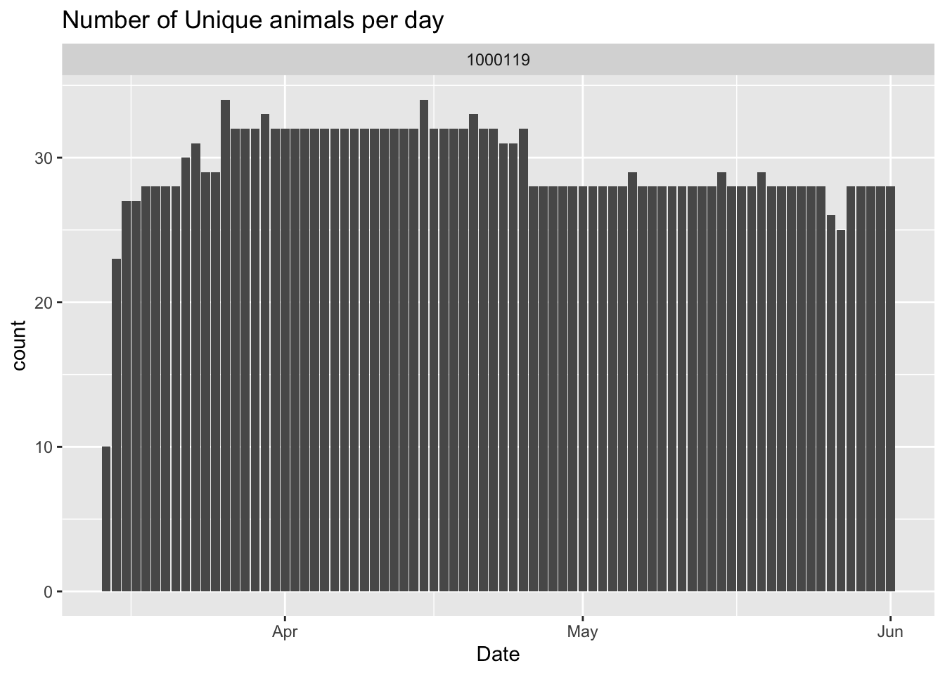
#convert start time to date
d.smart$Date=as.Date(d.smart$StartTime)

d.smart$RFID=stringr:: str_sub(d.smart$RFID,-6,-1)

#get a count on the number of good observations by each greenfeed by day
library(dplyr)
daily_good_data=d.smart %>% count(FeederID, Date, sort = TRUE)

daily_good_data=na.omit(daily_good_data)
ggplot(daily_good_data,aes(x=Date,y=n))+
  geom_bar(stat = 'identity')+
  facet_wrap(~FeederID)+
  ggtitle('Number of observations by SmartScale by day')+
  ylab('Number of daily observations')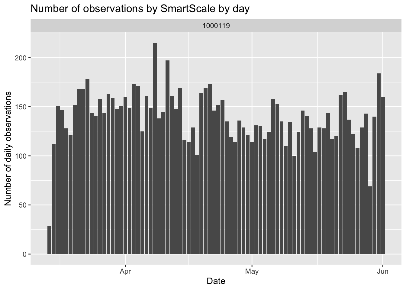
The smartscale data has a column named ‘Valid’ that flags potentially bad data in the system based on quantiles. The following plots show the bad data labeled as Valid = No for the entire dataset and for an individual animal.
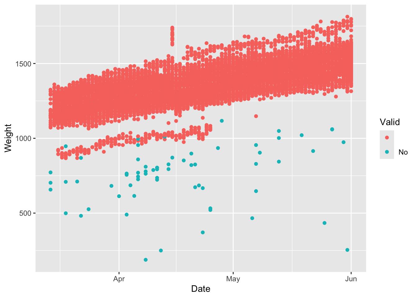
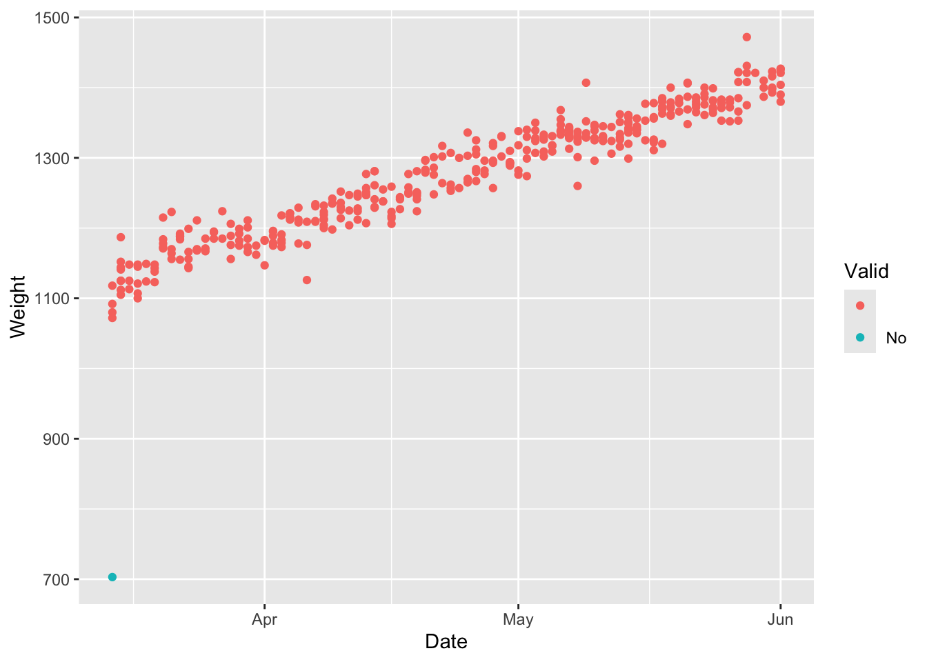
This next chunk of code will remove the observations that are not valid and replot the data.
#Remove not valid points
d.smart=subset(d.smart,Valid!='No')
#plot animal weight by date
ggplot(d.smart,aes(x=Date,y=Weight))+
  geom_point()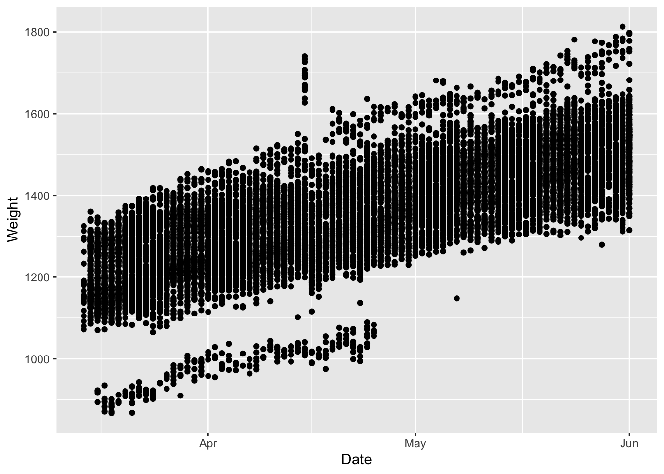
2.3.1 Further Data Cleaning and Filtering
This next code chunk will add day of trial to the dataframe which will help for calculating average daily gain (ADG)
# Add days to data
d.tdays = data.table(Date = seq.Date(from = as.Date(min(d.smart$Date)),
                                     to = as.Date(max(d.smart$Date)), by = 1),
                     tday = as.numeric(seq(from = 0,
                                           to = difftime(max(d.smart$Date), min(d.smart$Date), units = "days"))))
d.smart = d.tdays[d.smart, on = 'Date']
d.smart[, Weight:= as.numeric(Weight)]
d.smart[, RFIDTag := as.character(RFIDTag)]
In addition to flagging the data as valid or not valid, Parsons et al., 2023 proposed an additional method using robust regression to remove potentially bad data from in pasture weighing systems. We will apply that method below (Parsons et al. 2023).
# Filter Spurious weights using robust regression (Parsons et al., 2023)
m.rob = rlm(Weight ~ RFIDTag + tday, data = d.smart)
d.smrtrob = data.table(FeederID = d.smart$FeederID,
                       RFIDTag = d.smart$RFIDTag,
                       Date = d.smart$Date,
                       tday = d.smart$tday,
                       StartTime = d.smart$StartTime,
                       Duration = d.smart$Duration,
                       Weight = d.smart$Weight,
                       resid = m.rob$residuals,
                       hwt = m.rob$w)

## Assign outliers
d.smrtrob[, Outlier := fifelse(hwt > 0.99, 'In Range','Outlier')]

ggplot(subset(d.smrtrob,RFIDTag=='679563'),aes(x=Date,y=Weight,color=Outlier))+
  geom_point()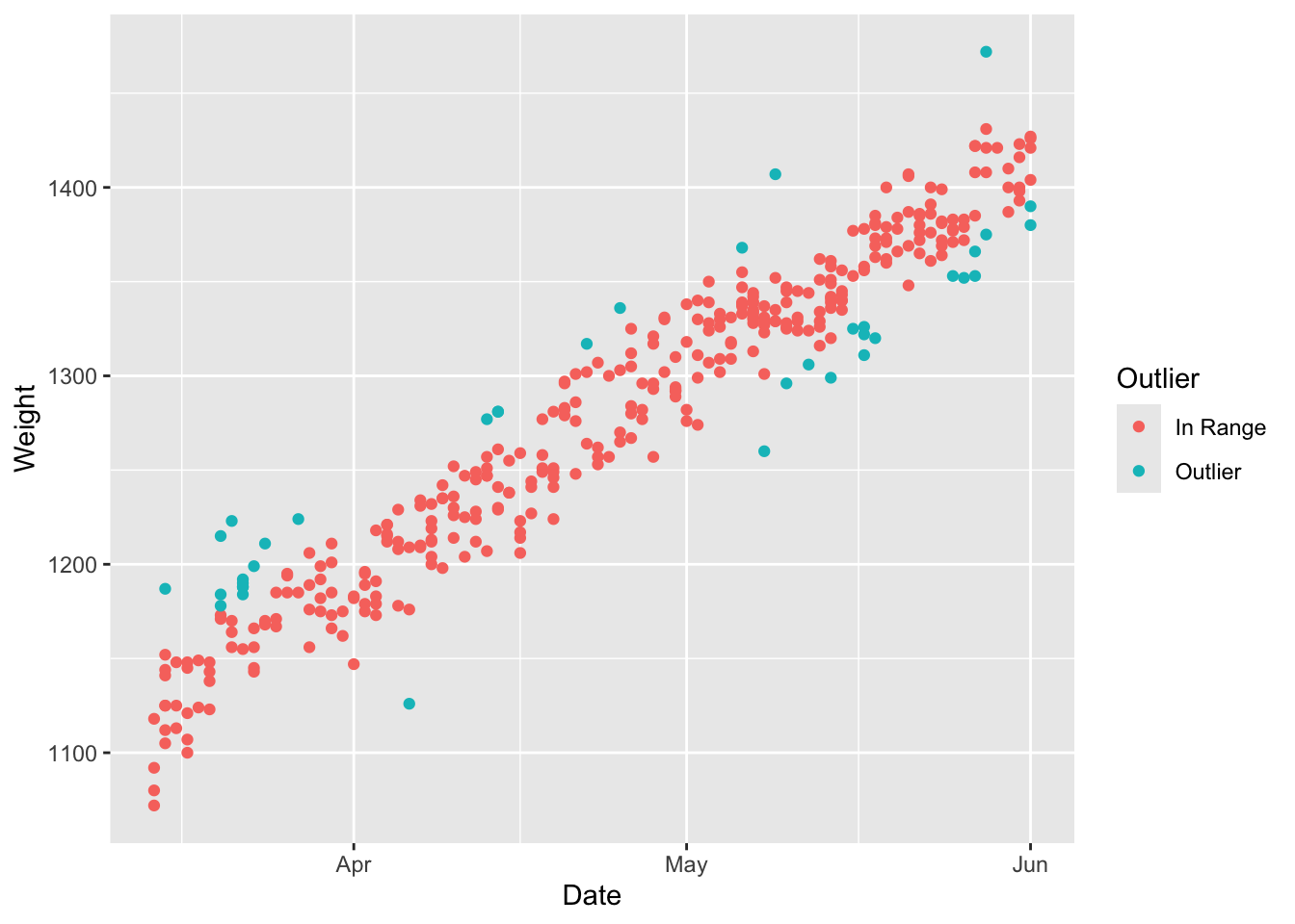
Using the table function we will get the number of daily weights for each individual animal. We can see that several tags only have a few observations while others have hundreds. These are could be test tags that were used to test the scales or had animals that infrequently used the equipement. The code below will delete individual tags with less than 6 observations.
##
## 030197 030226 030296 030312 605891 605892 605893 605896 605899 679558 679559 679560 679563 679572 679573 679590 679591 679593
##      6      1      2      1    242    255    365    354    326    281    242    243    337     70     57    400    231    229
## 679594 679596 679605 679608 679612 679617 679619 679622 679629 679633 679635 679663 679795 679814 679817 679822 680396 680410
##    340    318    132    333    144    337    338    212    175    241    293      2      4      2      6      2    243    260
## 680411 680412 680413 680414 828028 828031 828038
## 334 257 269 305 216 296 340##
## 030197 605891 605892 605893 605896 605899 679558 679559 679560 679563 679572 679573 679590 679591 679593 679594 679596 679605
## 6 242 255 365 354 326 281 242 243 337 70 57 400 231 229 340 318 132
## 679608 679612 679617 679619 679622 679629 679633 679635 679817 680396 680410 680411 680412 680413 680414 828028 828031 828038
## 333 144 337 338 212 175 241 293 6 243 260 334 257 269 305 216 296 3402.4 Animal Performance
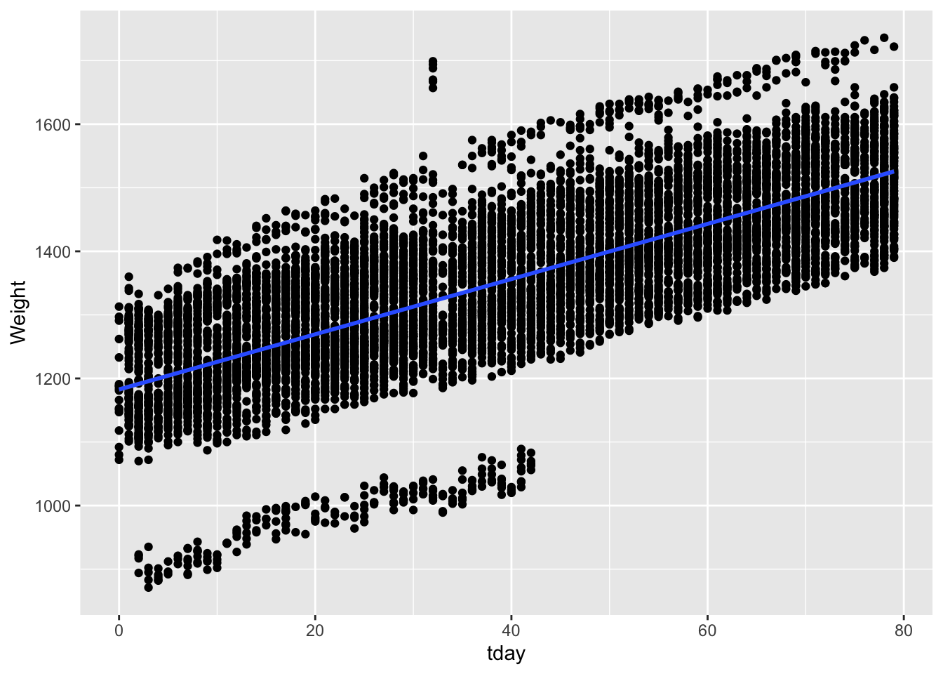
Next we want to calculate the average daily gain. To do so we can fit a linear regression to get a model for to estimate weight by day of trial. If we wanted to fit a linear model to the entire herd we can do so using all available data with Weight as our y and trial day as our x. The code below fits this linear model.
##
## Call:
## lm(formula = Weight ~ tday, data = d.smart)
##
## Residuals:
##     Min      1Q  Median      3Q     Max
## -336.93  -51.31   -8.48   62.83  377.41
##
## Coefficients:
##              Estimate Std. Error t value Pr(>|t|)
## (Intercept) 1.183e+03  1.883e+00   628.0   <2e-16 ***
## tday        4.342e+00  4.207e-02   103.2   <2e-16 ***
## ---
## Signif. codes:  0 '***' 0.001 '**' 0.01 '*' 0.05 '.' 0.1 ' ' 1
##
## Residual standard error: 88.14 on 9025 degrees of freedom
## Multiple R-squared:  0.5414, Adjusted R-squared:  0.5414
## F-statistic: 1.065e+04 on 1 and 9025 DF,  p-value: < 2.2e-16
We can see that the intercept of the model is 536, which would equate to our average starting weight for the herd and the slope is 1.96 which would equate to our average daily gain (ADG). Plotting it we can see the relationship.
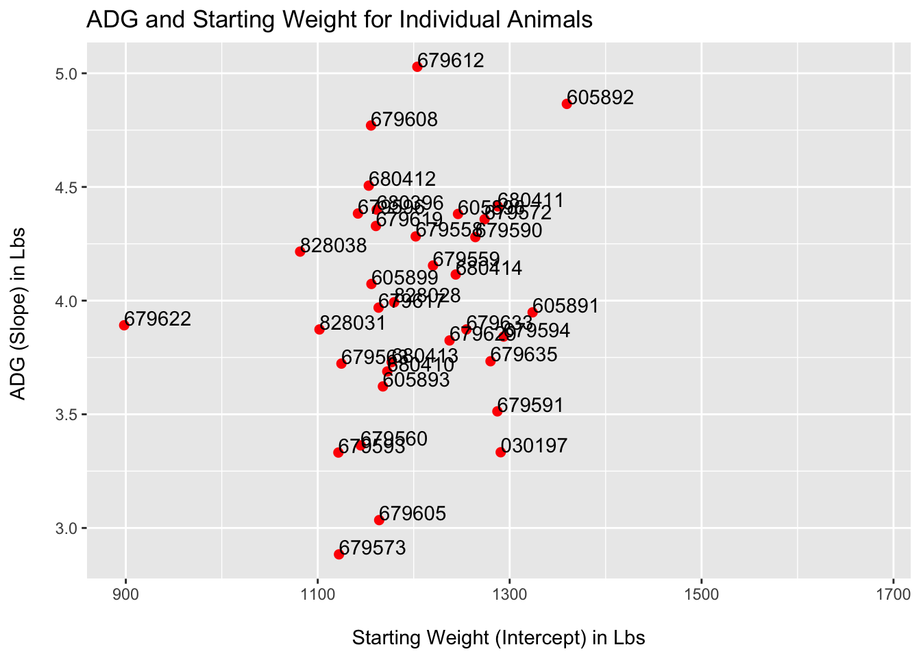
Though herd level ADG is important, using precision data we can also look at individual animal ADG. To do so we need to run a linear model for each individual animal. The code below will loop through each individual animal, subset the data based on RFID tag, create a linear model as above, extract the slope and intercept for the model, and save them in a new dataframe that contains the RFIDtag, slope, and intercept for each individual animal.
ADG_individual=data.frame()


for (i in 1:length(unique(d.smart$RFIDTag))){

    sublm=subset(d.smart,RFIDTag==unique(d.smart$RFIDTag)[i])
    mod=lm(sublm$Weight~sublm$tday)
    int= mod$coefficients[1]
    slope=mod$coefficients[2]


    sub_df=data.frame(unique(sublm$RFIDTag),int,slope)
    ADG_individual=rbind(ADG_individual,sub_df)
}

row.names(ADG_individual) <- NULL
Plotting the data we can see the slope and intercept for each animal with the RFID tag.
colnames(ADG_individual)=c('RFIDTag','Intercept','Slope')


ggplot(ADG_individual,aes(x=Intercept,y=Slope,label=RFIDTag))+
  geom_point(size=2,color='Red')+
  geom_text(hjust=0, vjust=0)+
  ggtitle('ADG and Starting Weight for Individual Animals')+
  xlab("\nStarting Weight (Intercept) in Lbs")+
  ylab('ADG (Slope) in Lbs \n')